1. Introduction to CAST 1.0.0

Introduction

Background

One key task in environmental science is obtaining information of environmental variables continuously in space or in space and time, usually based on remote sensing and limited field data. In that respect, machine learning algorithms have been proven to be an important tool to learn patterns in nonlinear and complex systems. However, standard machine learning applications are not suitable for spatio-temporal data, as they usually ignore the spatio-temporal dependencies in the data. This becomes problematic in (at least) two aspects of predictive modelling: Overfitted models as well as overly optimistic error assessment (see Meyer et al 2018 or Meyer et al 2019 ). To approach these problems, CAST supports the well-known caret package (Kuhn 2018 to provide methods designed for spatio-temporal data.

This tutorial shows how to set up a spatio-temporal prediction model that includes objective and reliable error estimation. It further shows how spatio-temporal overfitting can be detected by comparison between validation strategies. It will be shown that certain variables are responsible for the problem of overfitting due to spatio-temporal autocorrelation patterns. Therefore, this tutorial also shows how to automatically exclude variables that lead to overfitting with the aim to improve the spatio-temporal prediction model.

In order to follow this tutorial, I assume that the reader is familiar with the basics of predictive modelling nicely explained in Kuhn and Johnson 2013 as well as machine learning applications via the caret package.

How to start

To work with the tutorial, first install the CAST package and load the library:

#install.packages("CAST")
library(CAST)

If you need help, see

help(CAST)

Example of a typical spatio-temporal prediction task

The example prediction task for this tutorial is the following: we have a set of data loggers distributed over a farm, and we want to map soil moisture, based on a set of spatial and temporal predictor variables. We will use Random Forests as a machine learning algorithm in this tutorial.

Description of the example dataset

To do so, we will work with data of the sPlotOpen vegetation database. #TODO

data(splotdata)
head(splotdata)

##   PlotObservationID   GIVD_ID   Country                      Biome
## 1              1955 SA-AR-002 Argentina Dry tropics and subtropics
## 2              1956 SA-AR-002 Argentina Dry tropics and subtropics
## 3              1958 SA-AR-002 Argentina Dry tropics and subtropics
## 4              1960 SA-AR-002 Argentina Dry tropics and subtropics
## 5              1961 SA-AR-002 Argentina Dry tropics and subtropics
## 6              1963 SA-AR-002 Argentina Dry tropics and subtropics
##   Species_richness    bio_1    bio_4 bio_5 bio_6    bio_8    bio_9 bio_12
## 1               52 17.65000 463.9651  30.5   3.6 23.25000 11.70000    760
## 2               56 17.35417 459.5525  30.1   3.5 22.91667 11.46667    731
## 3               65 18.31667 473.3216  31.4   4.2 24.03333 12.25000    810
## 4               50 18.04167 485.8116  31.2   4.2 23.93333 11.81667    842
## 5               45 18.79167 478.4959  32.0   4.4 24.48333 12.65000    853
## 6               31 18.92083 478.9594  32.2   4.5 24.61667 12.76667    842
##   bio_13 bio_14   bio_15 elev             geometry
## 1    119      9 68.89403  416 -63.86056, -30.29722
## 2    115      9 68.93396  468 -63.94722, -30.37222
## 3    129     12 66.87429  232 -63.66278, -30.37806
## 4    140     13 65.54655  129 -63.32139, -30.98694
## 5    134     12 68.29005  231 -63.55694, -29.89889
## 6    133     12 68.72808  243 -63.53972, -29.75833

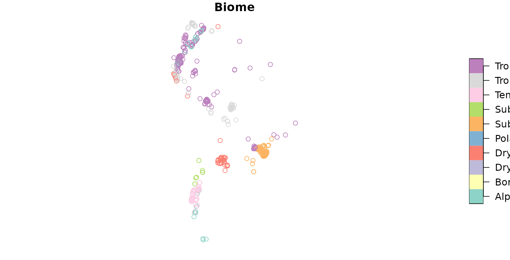
To get an impression on the spatial properties of the dataset, let’s have a look on the spatial distribution of the vegetation plots in South America:

library(sf)
plot(splotdata[,"Biome"])

#...or plot the data with mapview:
library(mapview)
mapviewOptions(basemaps = c("Esri.WorldImagery"))
mapview(splotdata)

Model training and prediction

To start with, lets use this dataset to create a “default” Random Forest model that predicts species richness based on some predictor variables. To keep computation time at a minimum, we don’t include hyperparameter tuning (hence mtry was set to 2) which is reasonable as Random Forests are comparably insensitive to tuning.

library(caret)
predictors <- c("bio_1", "bio_4", "bio_5", "bio_6",
                "bio_8", "bio_9", "bio_12", "bio_13",
                "bio_14", "bio_15", "elev")

# to use the data for model training we have to get rid of the geometry column
trainDat <- st_drop_geometry(splotdata)

set.seed(10)
model <- train(trainDat[,predictors],trainDat$Species_richness,
               method="rf",tuneGrid=data.frame("mtry"=2),
               importance=TRUE,ntree=50,
               trControl=trainControl(method="cv",number=3))

Based on the trained model we can make spatial predictions of species richness. To do this we load a multiband raster that contains spatial data of all predictor variables for Chile. We then apply the trained model on this data set.

library(terra)
predictors_sp <- rast(system.file("extdata", "predictors_chile.tif",package="CAST"))
prediction <- predict(predictors_sp,model,na.rm=TRUE)
plot(prediction)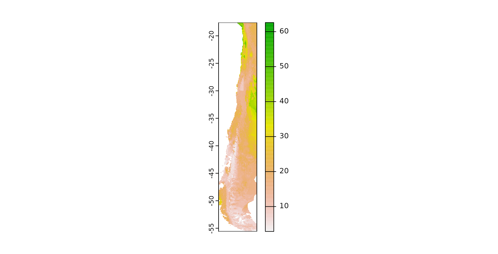

The result is a spatially comprehensive map of the species richness of Chile. We see that simply creating a map using machine learning and caret is an easy task, however accurately measuring its performance is less simple. Though the map looks good on a first sight we now have to follow up with the question of how accurate this map is, hence we need to ask how well the model is able to map species richness.

From a visible inspection it is noticeable that the model produces a strange linear feature in the south west of Chile which looks suspicious. But let’s come back to this later and first focus on a statistical validation of the model.

Cross validation strategies for spatio-temporal data

Among validation strategies, k-fold cross validation (CV) is popular to estimate the performance of the model in view to data that have not been used for model training. During CV, models are repeatedly trained (k models) and in each model run, the data of one fold are put to the side and are not used for model training but for model validation. In this way, the performance of the model can be estimated using data that have not been included in the model training.

The Standard approach: Random k-fold CV

In the example above we used a random k-fold CV that we defined in caret’s trainControl argument. More specifically, we used a random 3-fold CV. Hence, the data points in our dataset were RANDOMLY split into 3 folds. To assess the performance of the model let’s have a look on the output of the Random CV:

model

## Random Forest 
## 
## 703 samples
##  11 predictor
## 
## No pre-processing
## Resampling: Cross-Validated (3 fold) 
## Summary of sample sizes: 470, 469, 467 
## Resampling results:
## 
##   RMSE      Rsquared   MAE     
##   25.75544  0.6651004  15.08417
## 
## Tuning parameter 'mtry' was held constant at a value of 2

We see that species richness could be modelled with a R² of 0.66 which indicates a good fit of the data. Sounds good, but unfortunately, the random k fold CV does not give us a good indication for the map accuracy. Random k-fold CV means that each of the three folds (with the highest certainty) contains data points from each known location. Therefore, a random CV cannot indicate the ability of the model to make predictions beyond the location of the training data (i.e. to map species richness). Since our aim is to map species richness, we rather need to perform a target-oriented validation which validates the model in view to spatial mapping.

Target-oriented validation

We are not interested in the model performance in view to random subsets of our vegetation plots, but we need to know how well the model is able to make predictions for areas without reference samples. To find this out, we need to repeatedly leave larger spatial regions of one or more vegetation plots out and use them as test data during CV.

To do this we first need to create meaningful folds rather than random folds. CAST’s function “CreateSpaceTimeFolds” is designed to provide index arguments used by caret’s trainControl. The index defines which data points are used for model training during each model run and reversely defines which data points are held back. Hence, using the index argument we can account for the dependencies in the data by leaving the complete data from one or more regions out (LLO CV), from one or more time steps out (LTO CV) or from data loggers and time steps out (LLTO CV). In this example we’re focusing on LLO CV, therefore we use the column “Biome” to define the location of a data logger and split the data into folds using this information. Analog to the random CV we split the data into five folds, hence five model runs are performed each leaving one fifth of all data loggers out for validation.

Note that several suggestions of spatial CV exist. What we call LLO here is just a simple example. See references in Meyer and Pebesma 2022 for some examples and have a look at Mila et al 2022 for the methodology implemented in the CAST function nndm.

set.seed(10)
indices <- CreateSpacetimeFolds(trainDat,spacevar = "Biome",
                                k=3)
set.seed(10)
model_LLO <- train(trainDat[,predictors],trainDat$Species_richness,
                   method="rf",tuneGrid=data.frame("mtry"=2), importance=TRUE,
                   trControl=trainControl(method="cv",
                                          index = indices$index))
model_LLO

## Random Forest 
## 
## 703 samples
##  11 predictor
## 
## No pre-processing
## Resampling: Cross-Validated (10 fold) 
## Summary of sample sizes: 532, 244, 630 
## Resampling results:
## 
##   RMSE      Rsquared   MAE     
##   28.34083  0.3674409  18.11776
## 
## Tuning parameter 'mtry' was held constant at a value of 2

By inspecting the output of the model, we see that in view to new locations, the R² is only 0.36 so the performance is much lower than expected from the random CV (R² = 0.66).

Apparently, there is considerable overfitting in the model, causing a good random performance but a poor performance in view to new locations. This might partly be attributed to the choice of variables where we must suspect that certain variables are misinterpreted by the model (see Meyer et al 2018 or [talk at the OpenGeoHub summer school 2019] (https://www.youtube.com/watch?v=mkHlmYEzsVQ)).

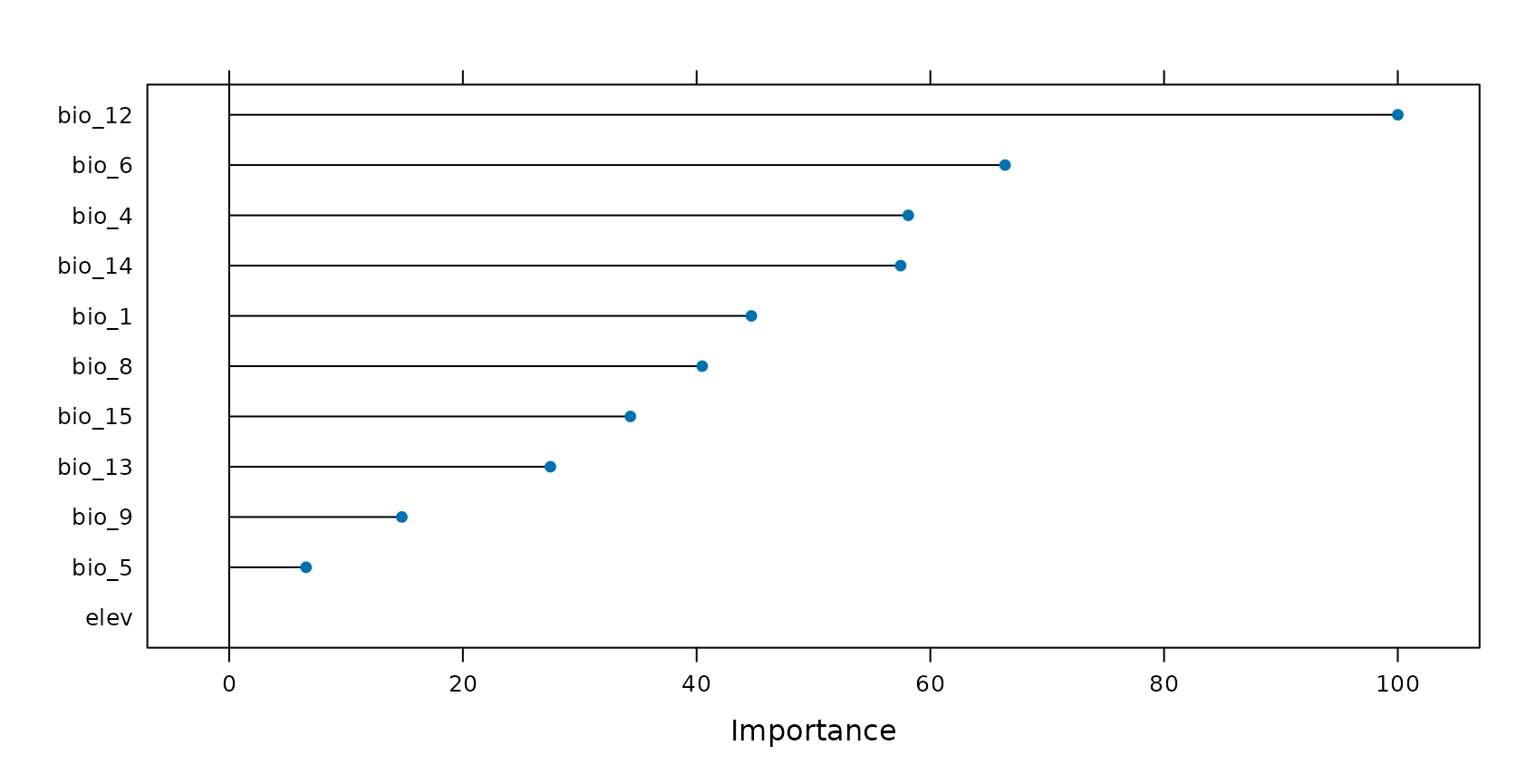
Let’s have a look at the variable importance ranking of Random Forest. Assuming that certain variables are misinterpreted by the algorithm we should be able to produce a higher LLO performance when such variables are removed. Let’s see if this is true…

plot(varImp(model_LLO))

Removing variables that cause overfitting

CAST’s forward feature selection (ffs) selects variables that make sense in view to the selected CV method and excludes those which are counterproductive (or meaningless) in view to the selected CV method. When we use LLO as CV method, ffs selects variables that lead in combination to the highest LLO performance (i.e. the best spatial model). All variables that have no spatial meaning or are even counterproductive won’t improve or even reduce the LLO performance and are therefore excluded from the model by the ffs.

ffs is doing this job by first training models using all possible pairs of two predictor variables. The best model of these initial models is kept. On the basis of this best model the predictor variables are iterativly increased and each of the remaining variables is tested for its improvement of the currently best model. The process stops if none of the remaining variables increases the model performance when added to the current best model.

So let’s run the ffs on our case study using R² as a metric to select the optimal variables. This process will take 1-2 minutes…

set.seed(12)
ffsmodel_LLO <- ffs(trainDat[,predictors],trainDat$Species_richness,metric="Rsquared",
                    method="rf", tuneGrid=data.frame("mtry"=2),
                    verbose=FALSE,ntree=50,
                    trControl=trainControl(method="cv",
                                           index = indices$index))
ffsmodel_LLO

## Selected Variables: 
## bio_1 bio_12 bio_6
## ---
## Random Forest 
## 
## 703 samples
##   3 predictor
## 
## No pre-processing
## Resampling: Cross-Validated (10 fold) 
## Summary of sample sizes: 532, 244, 630 
## Resampling results:
## 
##   RMSE      Rsquared   MAE     
##   26.70724  0.4240436  17.70666
## 
## Tuning parameter 'mtry' was held constant at a value of 2

ffsmodel_LLO$selectedvars

## [1] "bio_1"  "bio_12" "bio_6"

Using the ffs with LLO CV, the R² could be increased from 0.36 to 0.42. The variables that are used for this model are “bio_1”,“bio_12” and “bio_6”. All others are removed because they have (at least in this small example) no spatial meaning or are even counterproductive.

By plotting the results of ffs, we can visualize how the performance of the model changed depending on the variables being used:

plot(ffsmodel_LLO)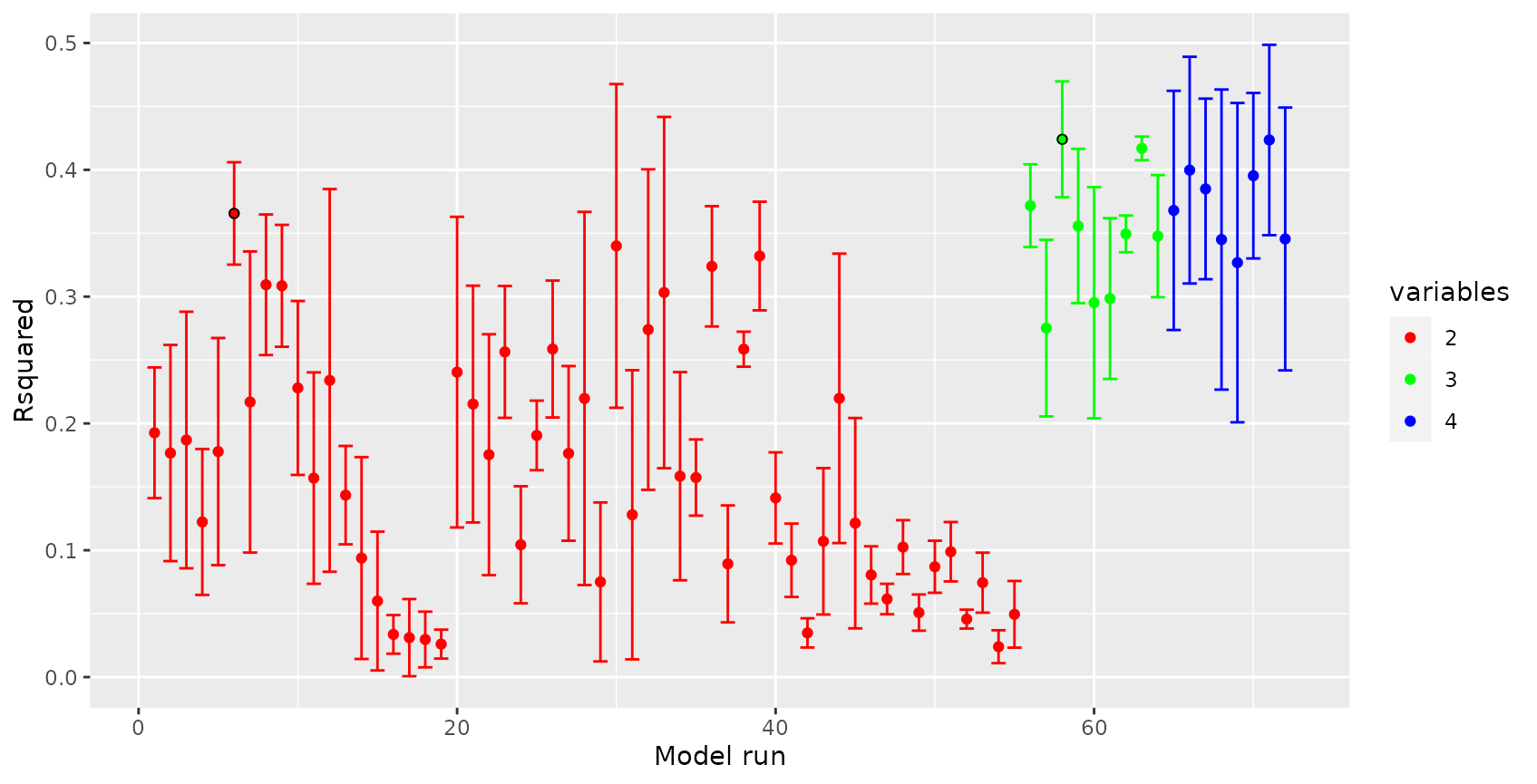

See that the best model using two variables led to an R² of slightly above 0.35. Using the third variable could slightly increase the R². Any further variable could not improve the LLO performance. Note that the R² features a high standard deviation regardless of the variables being used. This is due to the small dataset that was used which cannot lead to robust results.

What effect does the new model has on the spatial representation of species richness?

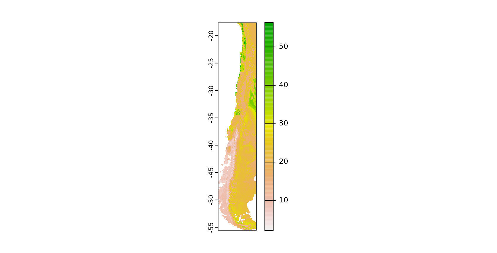
prediction_ffs <- predict(predictors_sp,ffsmodel_LLO,na.rm=TRUE)
plot(prediction_ffs)

Area of Applicability

Still it is required to analyse if the model can be applied to the entire study area of if there are locations that are very different in their predictor properties to what the model has learned from. See more details in the vignette on the Area of applicability and Meyer and Pebesma 2021.

### AOA for which the spatial CV error applies:
AOA <- aoa(predictors_sp,ffsmodel_LLO)

plot(prediction_ffs,main="prediction for the AOA \n(spatial CV error applied)")
plot(AOA$AOA,col=c("grey","transparent"),add=T)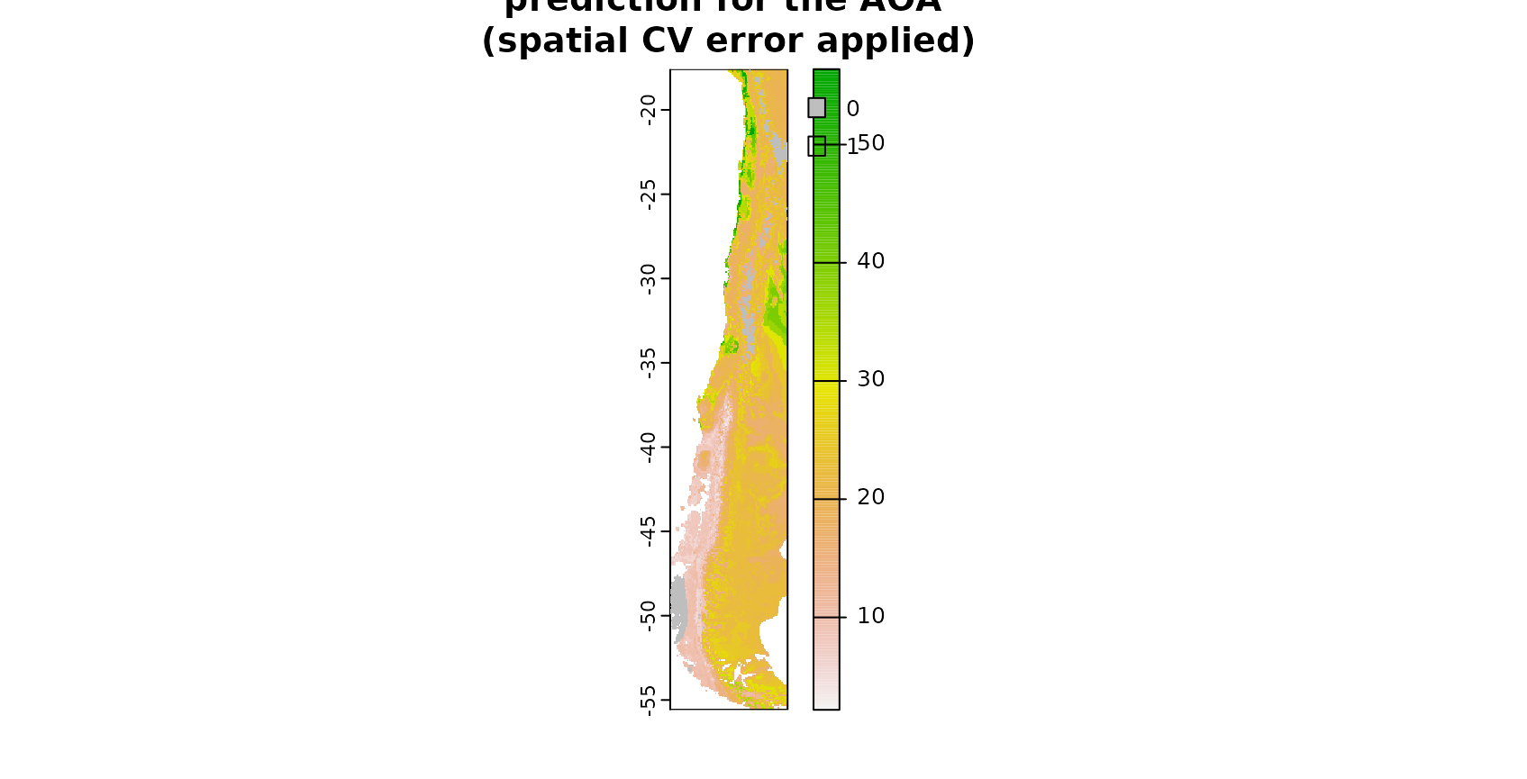

### AOA for which the random CV error applies:
AOA_random <- aoa(predictors_sp,model)
plot(prediction,main="prediction for the AOA \n(random CV error applied)")
plot(AOA_random$AOA,col=c("grey","transparent"),add=T)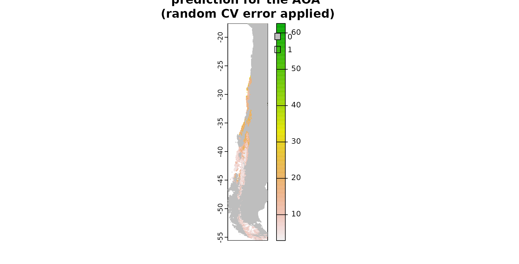

The figure shows in grey areas that are outside the area of applicability, hence predictions should not be considered for these locations. See tutorial on the AOA in this package for more information.

Conclusions

To conclude, the tutorial has shown how CAST can be used to facilitate target-oriented (here: spatial) CV on spatial and spatio-temporal data which is crucial to obtain meaningful validation results. Using the ffs in conjunction with target-oriented validation, variables can be excluded that are counterproductive in view to the target-oriented performance due to misinterpretations by the algorithm. ffs therefore helps to select the ideal set of predictor variables for spatio-temporal prediction tasks and gives objective error estimates.

Final notes

The intention of this tutorial is to describe the motivation that led to the development of CAST as well as its functionality. Priority is not on modelling species richness of Chile in the best possible way but to provide an example for the motivation and functionality of CAST that can run within a few minutes. Hence, only a very small subset of the entire sPlotOpen dataset was used. Keep in mind that due to the small subset the example is not robust and quite different results might be obtained depending on small changes in the settings.

Hanna Meyer

2023-11-18