3. Nearest neighbor distance matching Cross-validation in CAST

library("sf")
library("CAST")
library("caret")
library("gridExtra")
library("ggplot2")
library("knitr")

set.seed(1234)

Introduction

Cross-Validation (CV) is important for many tasks in the predictive mapping workflow, including feature selection (see CAST::ffs and CAST::bss), hyperparameter tuning, area of applicability estimation (see CAST::aoa), and error profiling (see CAST::errorProfiles). Moreover, in the unfortunate case where no independent samples are available to estimate the performance of the final predicted surfaces, it can be used as a last resort to obtain an estimate of the map error.

The objective of this vignette is to showcase the CV methods implemented in CAST. To do so, we will work with two datasets of annual average air temperature and fine Particulate Matter (PM\(_{2.5}\)) air pollution in continental Spain for 2019, for which several predictors have been collected. For more details, check our preprint where the dataset is described in detail.

# Read data
temperature <- read_sf("https://github.com/carlesmila/RF-spatial-proxies/raw/main/data/temp/temp_train.gpkg")
pm25 <- read_sf("https://github.com/carlesmila/RF-spatial-proxies/raw/main/data/AP/PM25_train.gpkg")
spain <- read_sf("https://github.com/carlesmila/RF-spatial-proxies/raw/main/data/boundaries/spain.gpkg")

# df versions
temperature_df <- as.data.frame(st_drop_geometry(temperature))
pm25_df <- as.data.frame(st_drop_geometry(pm25))

# Plot them
p1 <- ggplot() +
  geom_sf(data = spain, fill = "grey", alpha = 0.1) +
  geom_sf(data = temperature, aes(col = temp)) +
  scale_colour_distiller(palette = "RdYlBu") +
  theme_bw() +
  labs(col = "") +
  ggtitle("Average 2019 temperature (ºC)")
p2 <- ggplot() +
  geom_sf(data = spain, fill = "grey", alpha = 0.1) +
  geom_sf(data = pm25, aes(col = PM25)) +
  scale_colour_viridis_c(option = "cividis") +
  theme_bw() +
  labs(col = "") +
  ggtitle(expression(Average~2019~PM[2.5]~(mu*g/m^3)))
grid.arrange(p1, p2, nrow=2)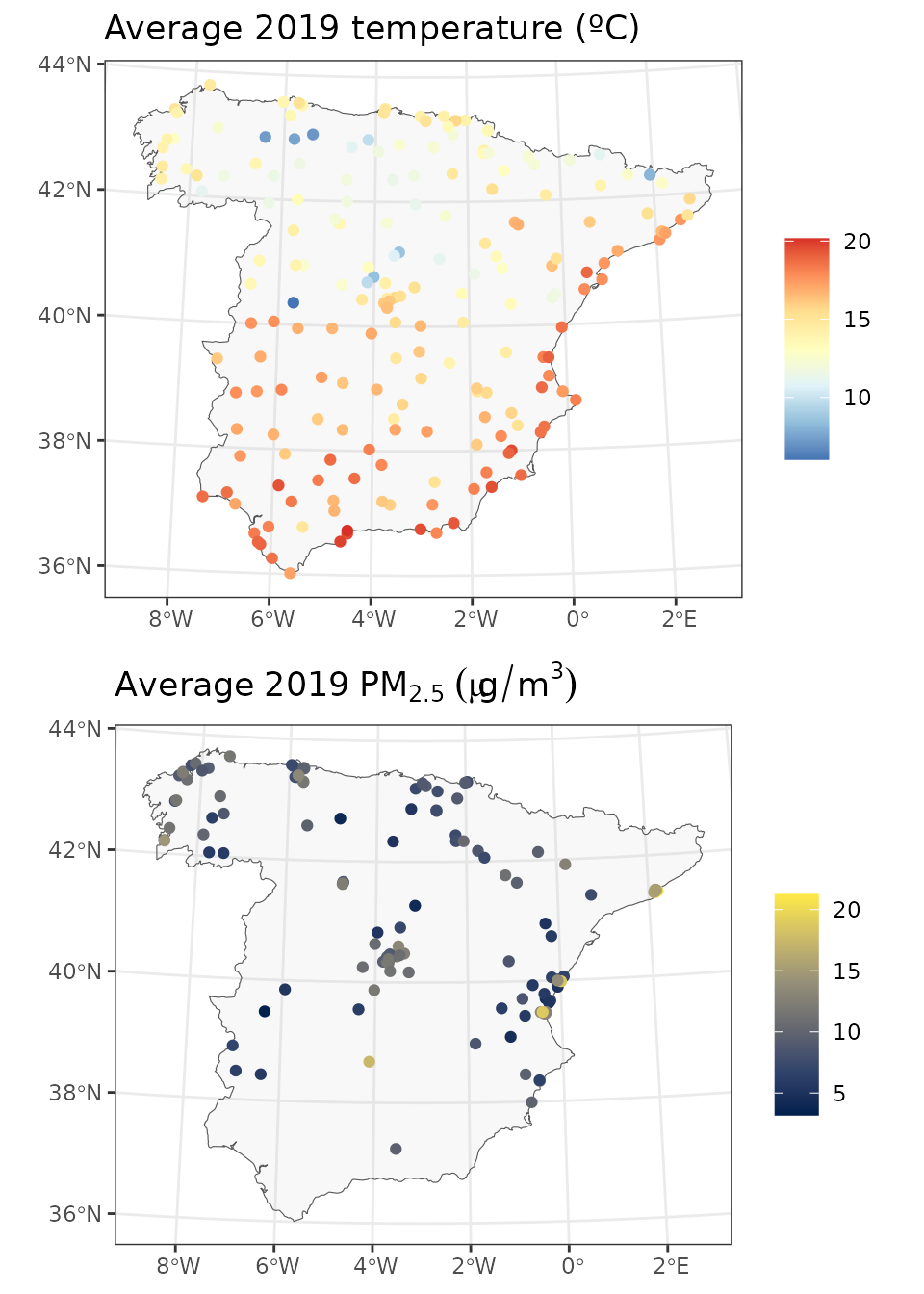

Looking at the two maps we can see that while air temperature stations are nicely distributed around the area of interest, air pollution stations are concentrated in specific regions.

Cross-validation in geographical space

In CAST, we deal with data that are indexed in space, i.e. data that are likely to present dependencies that do not comply with the assumptions of independence of standard CV methods such as Leave-One-Out (LOO) CV or k-fold CV. Several CV approaches have been proposed to try to deal with the dependency between the train and test data during CV, being spatial blocking and buffering two of the most used strategies. However, the CV methods included in CAST propose strategies that are not focused on ensuring independence, but that are rather prediction-oriented: we assess the predictive conditions found when using a model for a specific prediction task, and implement CV methods that aim to match them.

And how can we define these conditions? We have different options: we could consider the geographical space by focusing on the spatial locations of the training and prediction points. Another possibility is to consider the feature space, i.e. the covariate values both in the train and prediction set. There are yet other possibilities, such as space-time or a mixture of geographical and feature space. For now, though, let’s focus on the geographical space first.

Evaluation of spatial predictive conditions

First of all, let’s see what we mean by “predictive conditions” in practice. In the geographical space, we consider predictive conditions in terms of geographical nearest neighbour distances between prediction and training locations. In CAST, the distribution of such distances can be easily explored using the CAST::geodist function. CAST::geodist not only computes the distribution of nearest neighbour distances between 1) prediction and training points (prediction-to-sample), but also between 2) test points and training points during a LOO CV (sample-to-sample), 3) test points and training points during a given CV configuration (CV-distances).

Ideally, we would like the distribution of distances during CV to resemble as much as possible the distribution found during the prediction, since only then will predictive conditions be well-reflected during our CV. Let’s see this in practice for our environmental datasets and a random 5-fold CV, where we set the modeldomain to be the polygon of the study area from which prediction points are regularly sampled:

# Random 5-fold CV
fold5_temp <- createFolds(1:nrow(temperature), k=5, returnTrain=FALSE)
fold5_pm25 <- createFolds(1:nrow(pm25), k=5, returnTrain=FALSE)

# Explore geographic predictive conditions
predcond_temp <- geodist(temperature, modeldomain = spain, cvfolds = fold5_temp)
predcond_pm25 <- geodist(pm25, modeldomain = spain, cvfolds = fold5_pm25)

# Plot density functions
p1 <- plot(predcond_temp) + ggtitle("Temperature")
p2 <- plot(predcond_pm25) + ggtitle(expression(PM[2.5]))
grid.arrange(p1, p2, nrow=2)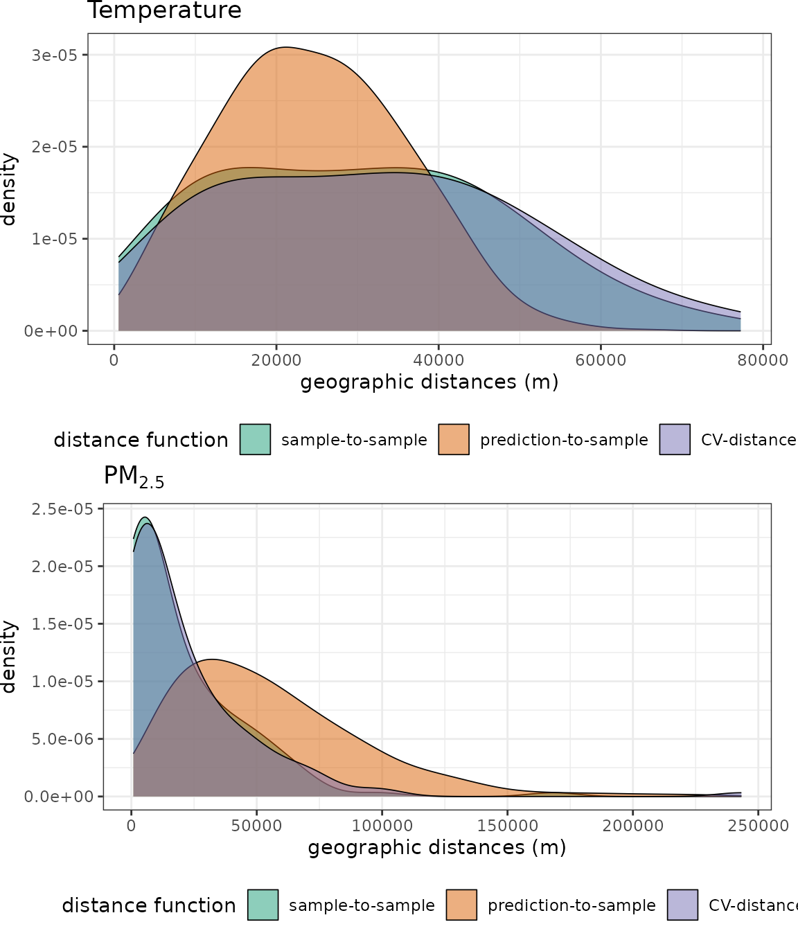

We see that, for temperature, although the distribution of geographical distances during CV vs. during prediction do not exactly match, the overlap between the two is substantial. In the PM\(_{2.5}\) case, however, the clustering of the stations make prediction-to-sample distances to be much longer that those found during CV. In other words, there are parts of the prediction area that do not have a PM\(_{2.5}\) station nearby, while this does not happen nearly as often during a random 5-fold CV.

Before we jump into the CV methods included in CAST, it is worth considering an alternative visualization of the distance distributions using Empirical Cumulative Density Functions (ECDF) rather than their density functions. ECDFs express, for a given distance, the proportion of distances in the distribution that have a value equal or lower to that value. Working with ECDFs has the advantage of not having to choose any additional parameters to estimate the density function, and are one of the building blocks of our proposed methods.

# Plot ECDF functions
p1 <- plot(predcond_temp, stat = "ecdf") + ggtitle("Temperature")
p2 <- plot(predcond_pm25, stat = "ecdf") + ggtitle(expression(PM[2.5]))
grid.arrange(p1, p2, nrow=2)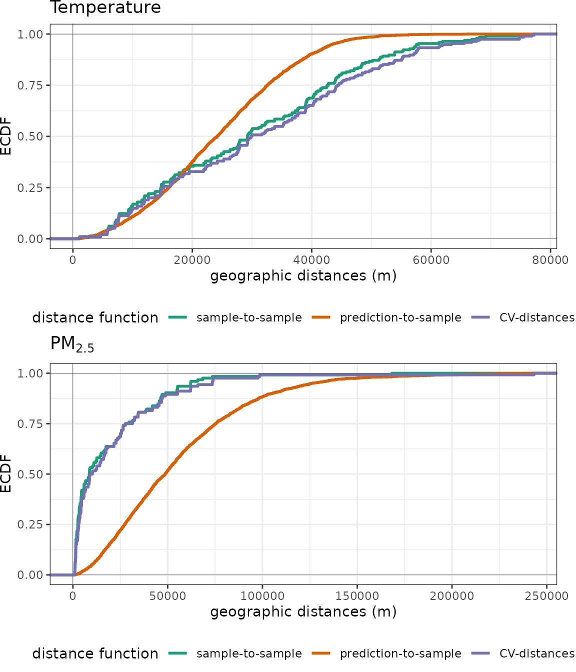

NNDM LOO CV for small datasets

The CV methods included in CAST are named Nearest Neighbour Distance Matching (NNDM), and their goal is to match the ECDF of nearest neighbour distances found during CV to the ECDF found during prediction we just saw in the last plots. For the geographical space, we will match geographical or Euclidean distances distributions depending on the CRS of the input data (in our examples we have a projected CRS so Euclidean distances are used).

The first of the two NNDM methods is NNDM LOO CV. It is a greedy, iterative algorithm that starts with a standard LOO CV and repetitively compares the prediction and CV ECDFs. When it finds that, for a given distance, the value of the ECDF during the CV is greater than the ECDF during the prediction, it excludes points in the neighbourhood of the sample being validated until a match is achieved. In practice, NNDM will exclude points whenever training data are clustered, while it will generalize to a standard LOO CV when data are random or regularly-distributed. All details regarding the algorithm and a simulation study evaluating its performance can be found in the article here (also listed at the end of the vignette).

Now, let’s run the NNDM LOO CV algorithm for our two datasets and check their output. Here, we use the polygon of Spain as modeldomain from which 1,000 are regularly sampled as prediction points. However, it is also be possible to pass to the function a set of prediction points previously defined, for example a set of raster cell centroids (check argument predpoints). We run it first for temperature:

temp_nndm <- nndm(temperature, modeldomain = spain, samplesize = 1000)
print(temp_nndm)

## nndm object
## Total number of points: 195
## Mean number of training points: 193.91
## Minimum number of training points: 191

plot(temp_nndm, type = "simple")

For temperature, we see that the ECDF of the NNDM LOO CV (CV-distances) is very similar to that of the LOO CV (sample-to-sample), as virtually no point is excluded from the training data during the CV. This is because the data are fairly regularly-distributed, and hence the ECDF during LOO is already lower than the prediction-to-sample ECDF. Now, we do the same for air pollution:

pm25_nndm <- nndm(pm25, modeldomain = spain, samplesize = 1000)
print(pm25_nndm)

## nndm object
## Total number of points: 124
## Mean number of training points: 118.74
## Minimum number of training points: 105

plot(pm25_nndm, type = "simple")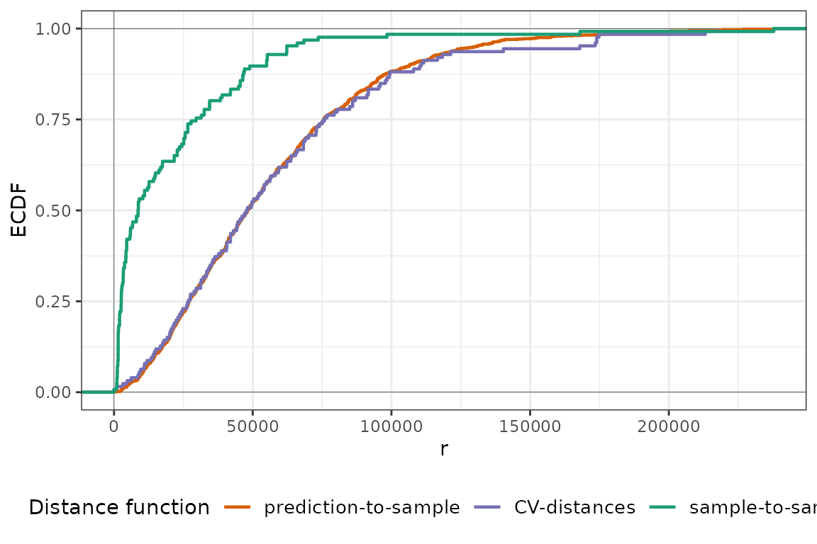

Here, things are quite different and many more points are excluded in order to match the prediction-to-sample ECDF successfully. As pointed out before, this is caused by the clustered pattern of the training samples. We can see how an iteration of NNDM LOO CV looks like by plotting it:

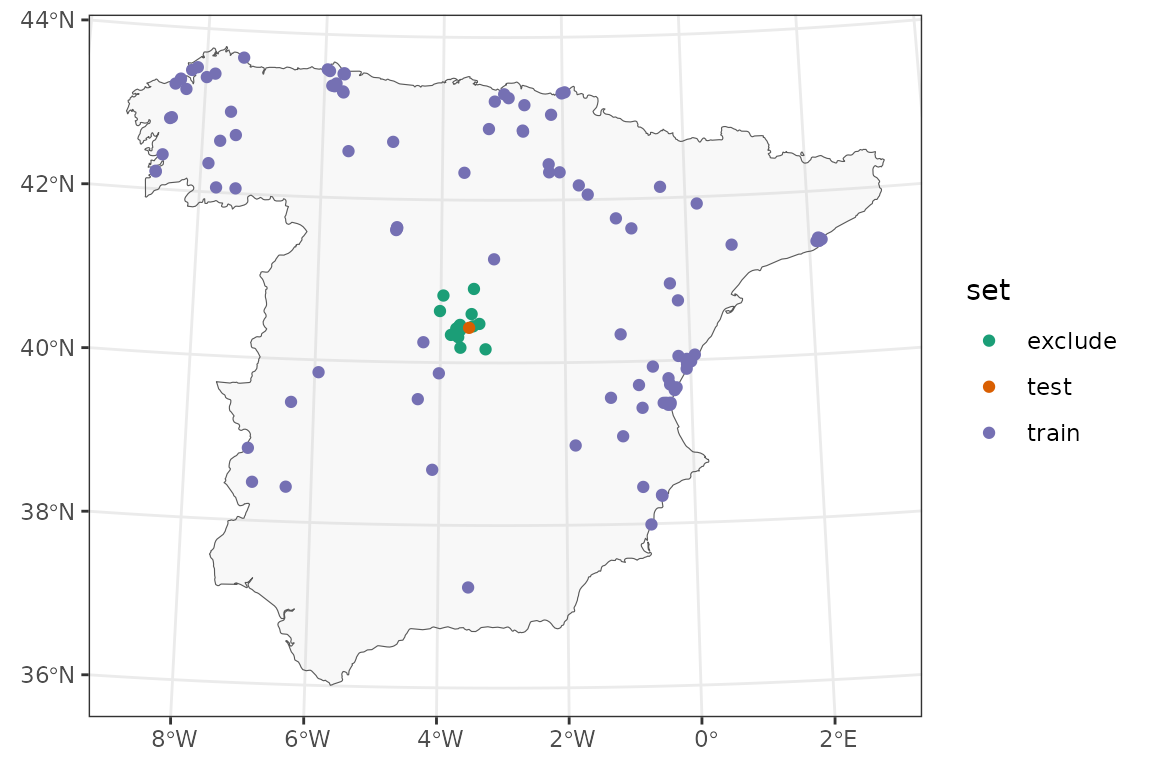
In this CV iteration, many samples around the point being validated are excluded. Now it’s time to fit the models and estimate their performance using 1) a standard LOO CV, and 2) NNDM LOO CV. Note that for all LOO methods, we need to use CAST::global_validation, which stacks all of the observed and the out-of-sample predicted values to get the relevant metrics in a single iteration.

First, we fit temperature models using a Digital Elevation Model (DEM), NDVI and Land Surface Temperature (LST) as predictors:

# LOO CV
temp_loo_ctrl <- trainControl(method="LOOCV", savePredictions=TRUE)
temp_loo_mod <- train(temperature_df[c("dem", "ndvi", "lst_day",  "lst_night")],
                      temperature_df[,"temp"],
                      method="rf", importance=FALSE,
                      trControl=temp_loo_ctrl, ntree=100, tuneLength=1)
temp_loo_res <- global_validation(temp_loo_mod)

# NNDM LOO CV
temp_nndm_ctrl <- trainControl(method="cv", 
                               index=temp_nndm$indx_train, # Obs to fit the model to
                               indexOut=temp_nndm$indx_test, # Obs to validate
                               savePredictions=TRUE)
temp_nndm_mod <- train(temperature_df[c("dem", "ndvi", "lst_day",  "lst_night")],
                       temperature_df[,"temp"],
                       method="rf", importance=FALSE,
                       trControl=temp_nndm_ctrl, ntree=100, tuneLength=1)
temp_nndm_res <- global_validation(temp_nndm_mod)

Next, we run PM\(_{2.5}\) models using population and road density, nighttime lights (NTL), and impervious surface (IMD) as predictors:

# LOO CV
pm25_loo_ctrl <- trainControl(method="LOOCV", savePredictions=TRUE)
pm25_loo_mod <- train(pm25_df[c("popdens", "primaryroads", "ntl", "imd")],
                      pm25_df[,"PM25"],
                      method="rf", importance=FALSE,
                      trControl=pm25_loo_ctrl, ntree=100, tuneLength=1)
pm25_loo_res <- global_validation(pm25_loo_mod)

# NNDM LOO CV
pm25_nndm_ctrl <- trainControl(method="cv", 
                               index=pm25_nndm$indx_train, # Obs to fit the model to
                               indexOut=pm25_nndm$indx_test, # Obs to validate
                               savePredictions=TRUE)
pm25_nndm_mod <- train(pm25_df[c("popdens", "primaryroads", "ntl", "imd")],
                       pm25_df[,"PM25"],
                       method="rf", importance=FALSE,
                       trControl=pm25_nndm_ctrl, ntree=100, tuneLength=1)
pm25_nndm_res <- global_validation(pm25_nndm_mod)

And we summarise the CV results in a table:

outcome	validation	RMSE	Rsquared	MAE
Temperature	LOO CV	0.86	0.91	0.65
Temperature	NNDM LOO CV	0.88	0.91	0.65
PM2.5	LOO CV	2.89	0.35	2.30
PM2.5	NNDM LOO CV	3.25	0.19	2.48

We can observe that the statistics for temperature models are almost the same for both CV methods since the NNDM algorithm did not detect any spatial clustering and thus returned a configuration almost identical to a standard LOO CV. However, for PM\(_{2.5}\), there are important differences between the performance estimated by the two CV methods, with NNDM LOO CV suggesting a much lower performance when the actual predictive conditions are taken into account.

kNNDM CV for medium and large datasets

One straightforward limitation of NNDM is sample size. Not only is it computationally expensive to run the NNDM algorithm for large sample sizes, but also the model fitting runtime becomes very long since, in a LOO CV, a model for each observation needs to be fit. To address this limitation, we developed a k-fold version of NNDM named kNNDM.

The goal of kNNDM is exactly the same as NNDM LOO CV: to match the ECDF of nearest neighbour distances during CV to the ECDF found during prediction. Nonetheless, the means to achieve it are different. In kNNDM, what we do is to use a clustering algorithm (k-means and agglomerative clustering are currently implemented) to cluster our samples data into \(q\) groups based on the coordinates, which are then merged into the final \(k\) folds. The smaller the \(q\), the stronger the spatial structure of the CV will be.

Among all candidate \(q\), we choose the fold configuration that offers the best match between the two ECDFs. We choose it based on the Wassterstein’s W statistic, which is the integral of the absolute value differences between the two ECDFs. The lower the W, the better the match. kNNDM will yield configurations with a spatial structure for clustered training samples while it will generalize to a standard random k-fold CV whenever the training data are random or regularly-distributed.

If you want to learn all the finer details of kNNDM and check our simulation study evaluating its performance, here is the link to the document (also listed at the end of the vignette). Now let’s apply kNNDM to our data! First, for temperature with the default clustering algorithm:

temp_knndm <- knndm(temperature, k = 5, modeldomain = spain, samplesize = 1000, 
                   clustering = "hierarchical", linkf = "ward.D2")
print(temp_knndm)

## knndm object
## Space: geographical
## Clustering algorithm: hierarchical
## Intermediate clusters (q): random CV
## W statistic: 9384.0966
## Number of folds: 5
## Observations in each fold:  39 39 39 39 39

plot(temp_nndm, type = "simple")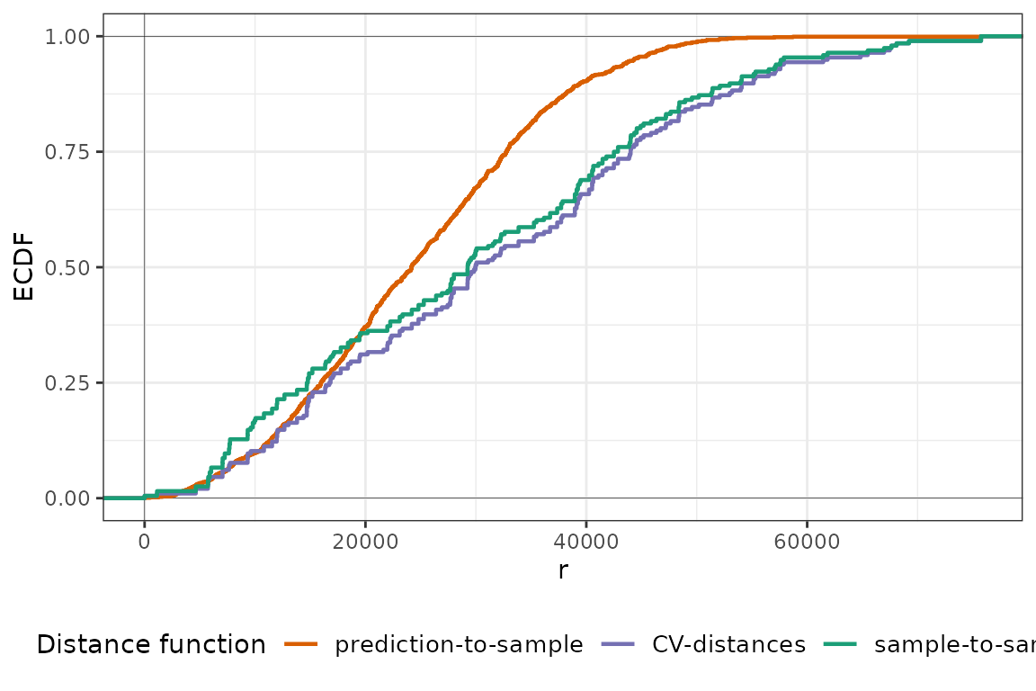

Similarly to NNDM LOO CV, kNNDM does not find any clustering and generalizes to a random k-fold CV. Now let’s see what happens in the PM\(_{2.5}\) dataset:

pm25_knndm <- knndm(pm25, k = 5, modeldomain = spain, samplesize = 1000, 
                    clustering = "hierarchical", linkf = "ward.D2")
print(pm25_knndm)

## knndm object
## Space: geographical
## Clustering algorithm: hierarchical
## Intermediate clusters (q): 46
## W statistic: 4919.5574
## Number of folds: 5
## Observations in each fold:  29 22 18 32 23

plot(pm25_knndm, type = "simple")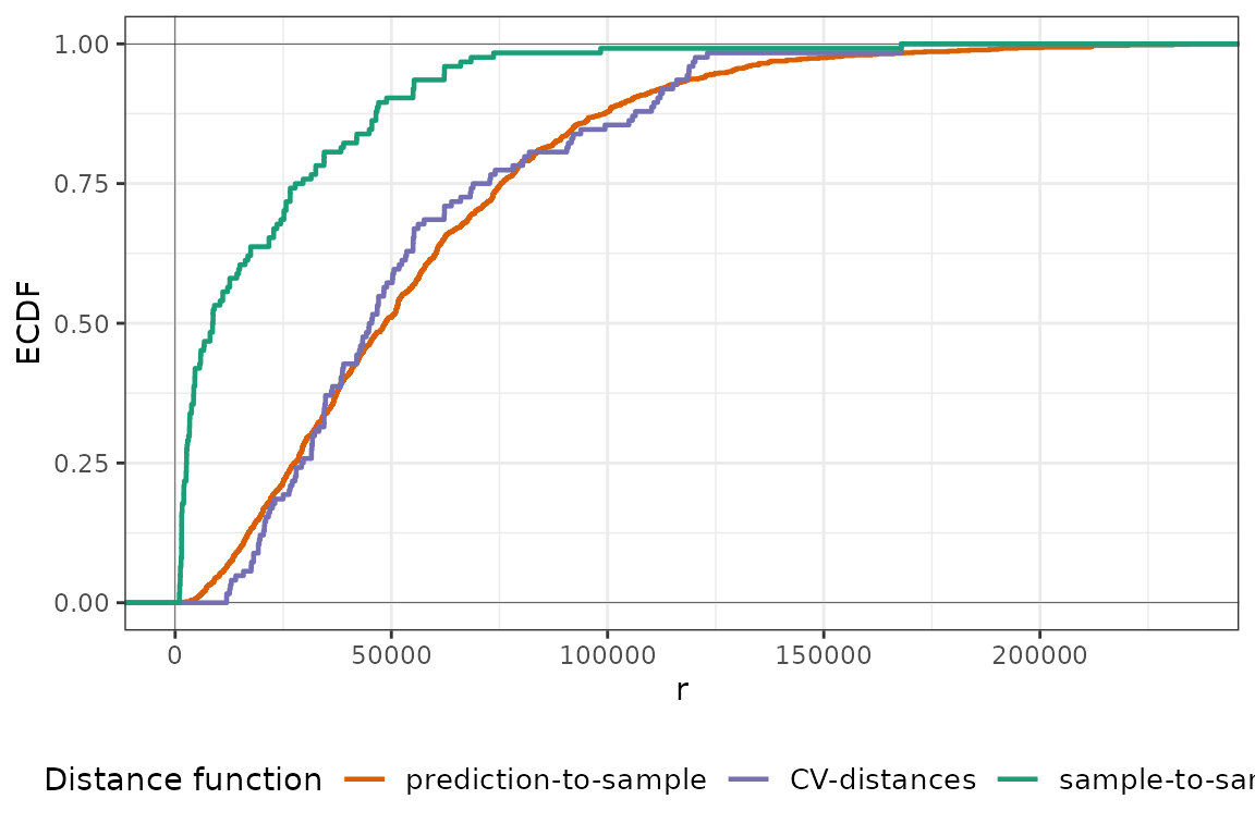

In this case, we do find clustered samples and kNNDM spatially clusters observations into folds as indicated by the number of intermediate clusters \(q\). With this kNNDM configuration, the match between the CV and the prediction distance distribution now seems to be quite good!

Another thing we can do is to check whether other clustering algorithms, or a different number of folds, might yield a better match. For example, let’s try using k-means clustering for the PM\(_{2.5}\) dataset:

pm25_knndm_v2 <- knndm(pm25, k = 5, modeldomain = spain, samplesize = 1000, 
                       clustering = "kmeans")
print(pm25_knndm_v2)

## knndm object
## Space: geographical
## Clustering algorithm: kmeans
## Intermediate clusters (q): 35
## W statistic: 5022.7072
## Number of folds: 5
## Observations in each fold:  21 23 17 40 23

We see that the W statistic is larger than before, hence indicating the quality of the match in this alternative kNNDM configuration is actually poorer, so we will stick to the first one. We can easily visualize the resulting 5-fold kNNDM configurations for both temperature and PM\(_{2.5}\):

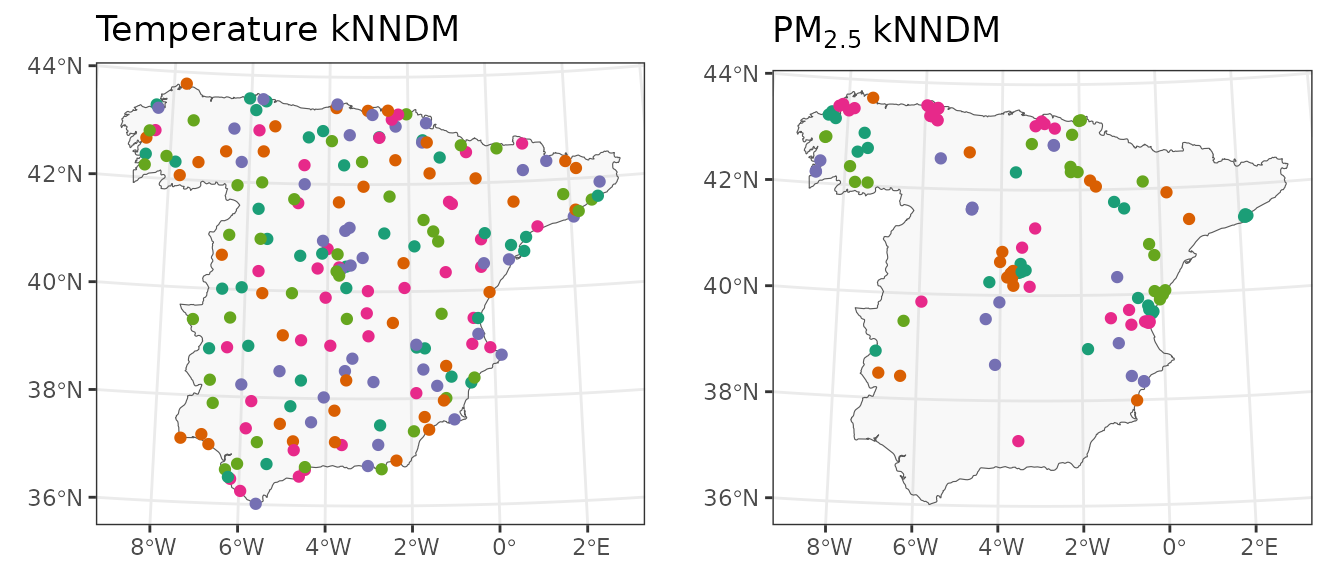
As we already knew, the 5-fold kNNDM configuration for temperature is random whereas the one for PM\(_{2.5}\) has a clear spatial pattern where observations close in space tend to be in the same fold.

Now, we can finally run our models (same predictors as before) and compare the results of a 5-fold random vs. kNNDM CV. To do so, we will still use the function CAST::global_validation to compute the statistics since 1) folds can be unbalanced and thus averaging might not weight all observations equally, and 2) we match the ECDF based on the whole distribution and not by fold. First, we run the temperature models:

# Random 5-fold CV
temp_rndmk_ctrl <- trainControl(method="cv", number=5, savePredictions=TRUE)
temp_rndmk_mod <- train(temperature_df[c("dem", "ndvi", "lst_day",  "lst_night")],
                      temperature_df[,"temp"],
                      method="rf", importance=FALSE,
                      trControl=temp_rndmk_ctrl, ntree=100, tuneLength=1)
temp_rndmk_res <- global_validation(temp_rndmk_mod)

# kNNDM 5-fold CV
temp_knndm_ctrl <- trainControl(method="cv", 
                                index=temp_knndm$indx_train,
                                savePredictions=TRUE)
temp_knndm_mod <- train(temperature_df[c("dem", "ndvi", "lst_day",  "lst_night")],
                        temperature_df[,"temp"],
                        method="rf", importance=FALSE,
                        trControl=temp_knndm_ctrl, ntree=100, tuneLength=1)
temp_knndm_res <- global_validation(temp_knndm_mod)

And the PM\(_{2.5}\) models:

# Random 5-fold CV
pm25_rndmk_ctrl <- trainControl(method="cv", number=5, savePredictions=TRUE)
pm25_rndmk_mod <- train(pm25_df[c("popdens", "primaryroads", "ntl", "imd")],
                        pm25_df[,"PM25"],
                        method="rf", importance=FALSE,
                        trControl=pm25_rndmk_ctrl, ntree=100, tuneLength=1)
pm25_rndmk_res <- global_validation(pm25_rndmk_mod)

# kNNDM 5-fold CV
pm25_knndm_ctrl <- trainControl(method="cv", 
                                index=pm25_knndm$indx_train,
                                savePredictions=TRUE)
pm25_knndm_mod <- train(pm25_df[c("popdens", "primaryroads", "ntl", "imd")],
                        pm25_df[,"PM25"],
                        method="rf", importance=FALSE,
                        trControl=pm25_knndm_ctrl, ntree=100, tuneLength=1)
pm25_knndm_res <- global_validation(pm25_knndm_mod)

And summarize the results in a table:

outcome	validation	RMSE	Rsquared	MAE
Temperature	Random 5-fold	0.92	0.90	0.68
Temperature	kNNDM 5-fold	0.89	0.91	0.65
PM2.5	Random 5-fold	2.92	0.34	2.32
PM2.5	kNNDM 5-fold	3.24	0.20	2.46

Here, we see the same pattern as in the LOO CV results. Since temperature data aren’t clustered, kNNDM CV has generalized to a random k-fold CV and thus results of both methods are very similar. This is not true for PM\(_{2.5}\), where kNNDM CV shows that once predictive conditions are taken into account, the estimated performance is lower.

Cross-validation in feature space

The ideas underlying NNDM methods in the geographical space can be transferred into the feature space with just a few tweaks. In the current version of CAST, we have implemented feature space experimental versions of CAST::nndm and CAST::knndm (see argument space= 'feature') and we are running validation analyses to verify their performance in a variety of settings. Stay tuned for a future version of the vignette for an overview of feature space NNDM CV methods and how to apply them to your datasets!

Carles Milà

2024-04-24