Collection of training data for remote sensing model building

Tutorial: EON Summer School 2023

#install.packages("devtools")
devtools::install_github("bleutner/RStoolbox")

Skipping install of 'RStoolbox' from a github remote, the SHA1 (ec6cac23) has not changed since last install.
  Use `force = TRUE` to force installation

library(sf)

Linking to GEOS 3.11.2, GDAL 3.6.2, PROJ 9.2.0; sf_use_s2() is TRUE

library(RStoolbox)

The legacy packages maptools, rgdal, and rgeos, underpinning the sp package,
which was just loaded, will retire in October 2023.
Please refer to R-spatial evolution reports for details, especially
https://r-spatial.org/r/2023/05/15/evolution4.html.
It may be desirable to make the sf package available;
package maintainers should consider adding sf to Suggests:.
The sp package is now running under evolution status 2
     (status 2 uses the sf package in place of rgdal)

library(raster)

Lade nötiges Paket: sp

library(knitr)
library(ggplot2)
library(rmarkdown)
library(patchwork)

Attache Paket: 'patchwork'

Das folgende Objekt ist maskiert 'package:raster':

    area

library(mapview)
library(kableExtra)
library(rmarkdown)
library("rprojroot")

Data sets

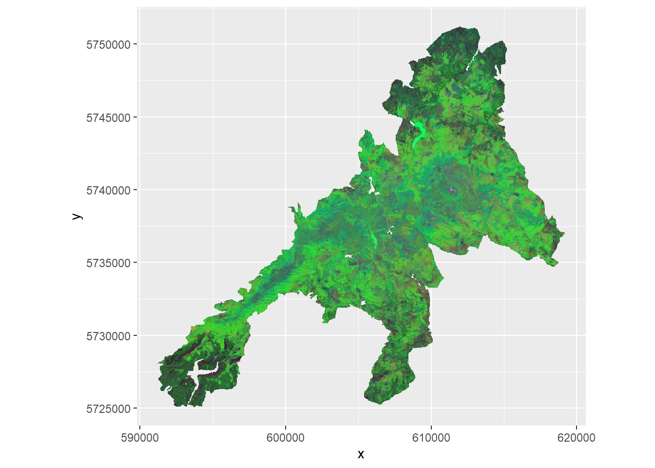
In this tutorial we will work with a Sentinel-2 scene from 18/06/2022 from the National Park, Harz. We will also use the boundary of the National Park to define our study area. Before we can start you may download the S2 Scene from the following link: S2-download. Place this file into the data folder of this tutorial.

# create a string containing the current working directory
wd=paste0(find_rstudio_root_file(),"/paul_tutorial/data/")

#Import the boundary of the n
np_boundary = st_transform(st_read(paste0(wd,"nlp-harz_aussengrenze.gpkg")),25832)

Reading layer `nlp-harz_aussengrenze' from data source 
  `C:\Users\49160\Documents\courses\EON\EON2023\paul_tutorial\data\nlp-harz_aussengrenze.gpkg' 
  using driver `GPKG'
Simple feature collection with 1 feature and 3 fields
Geometry type: MULTIPOLYGON
Dimension:     XY
Bounding box:  xmin: 591196.6 ymin: 5725081 xmax: 619212.6 ymax: 5751232
Projected CRS: WGS 84 / UTM zone 32N

s2  <- raster::brick(paste0(wd,"S2B_MSIL2A_20220618T102559_N0400_R10_resampled_harz_np.tif"))

names(s2)<-c('blue','green','red','vnir1','vnir2','vnir3','nir1','nir2','swir')

s2 <-raster::mask(s2,np_boundary)

Anaylsing the spectral variablity within the study area

If we have no access to prior information on our target variable in the study area we can use the spectral variability as a proxy for the variability of the target variable. By using the spectral variability as a sampling criterion we also ensure, that we cover the spectral range with our sampling.

Dimension reduction (PCA)

In a fist step we reduce the dimensions of the 9 Sentinel-2 bands while maintaining most of the information, using a principal component analysis (PCA).

#PCA
pca<-RStoolbox::rasterPCA(s2,nSamples = 5000, spca=TRUE )

ggRGB(pca$map,1,2,3, stretch="lin", q=0)

From the output of the PCA we see that we can capture 92% of the variability with the first two components. Thus we will only use the PC1 and PC2 for the subsequent analysis.

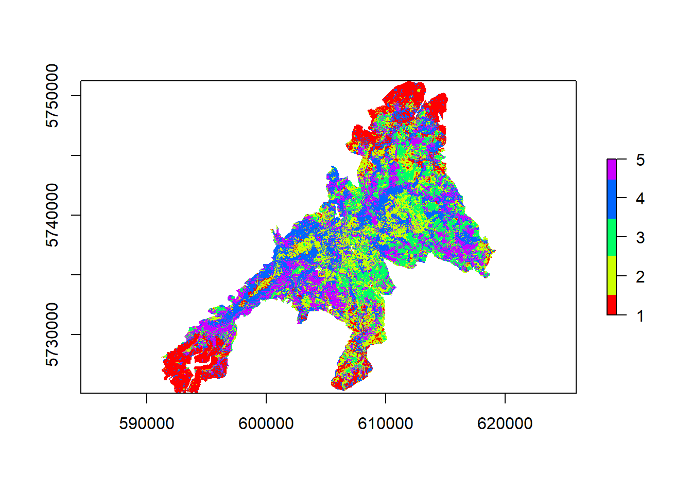
Unsupervised clustering

In the next step we run an unsupervised classification of the PC1 and PC2 to get a clustered map. For the unsupervised classification we need to take a decision on the number of classes/clusters to be created. Here we will take n=5 classes. However, depending on the target variable this value need to be adjusted.

set.seed(2222)
cluster <- unsuperClass(pca$map[[c('PC1','PC2')]], nSamples = 100, nClasses = 5, nStarts = 5)


## Plots
colors <- rainbow(5)
plot(cluster$map, col = colors, legend = TRUE, axes = TRUE, box =TRUE)

The map shows a clear spatial patterns related to the elevation, tree species and vitality status of the Nationalpark forests.

Create a stratified sample

In the next step we take a stratified random sample with \(n=10\) points from each of the 5 spectral classes.

samples <- sampleStratified(cluster$map,size = 10,na.rm=T,xy=T,sp=T)
samples$class <- as.factor(samples$class)
my.palette <- rainbow(5)
point.size <- 0.5

np.layer <- list("sp.polygons", as_Spatial(np_boundary))


spplot(samples,'class', col.regions = my.palette, sp.layout = np.layer,
    cex = point.size, main = "Stratified random sample for training")

We can now print the sample plot list as following:

kable(samples@data[c('x','y','class')], caption='Training plot list') %>%
  kable_styling(fixed_thead = T) %>% scroll_box(height = "400px")

Training plot list

x	y	class
611335	5750495	1
591385	5726975	1
611115	5748515	1
594375	5727165	1
606975	5729505	1
593825	5725735	1
607275	5726725	1
592305	5728525	1
611725	5749605	1
594425	5726745	1
604685	5737625	2
608785	5731095	2
605745	5739955	2
616025	5740945	2
595955	5728155	2
618615	5736595	2
609835	5734025	2
608895	5735735	2
606685	5739485	2
607075	5731635	2
613995	5742695	3
608905	5740045	3
608725	5739125	3
615335	5738535	3
608635	5741785	3
612345	5744955	3
607445	5740635	3
608705	5732285	3
611185	5737695	3
617605	5738225	3
614425	5747095	4
611505	5740905	4
611595	5737865	4
601625	5733415	4
598565	5734455	4
612825	5736295	4
604665	5735905	4
607065	5740135	4
601365	5734725	4
603315	5732365	4
607675	5738015	5
614105	5737465	5
596355	5730455	5
595455	5730655	5
601505	5736215	5
615025	5740415	5
610685	5744915	5
610185	5741695	5
613605	5744835	5
612755	5746185	5

Implement a plot design

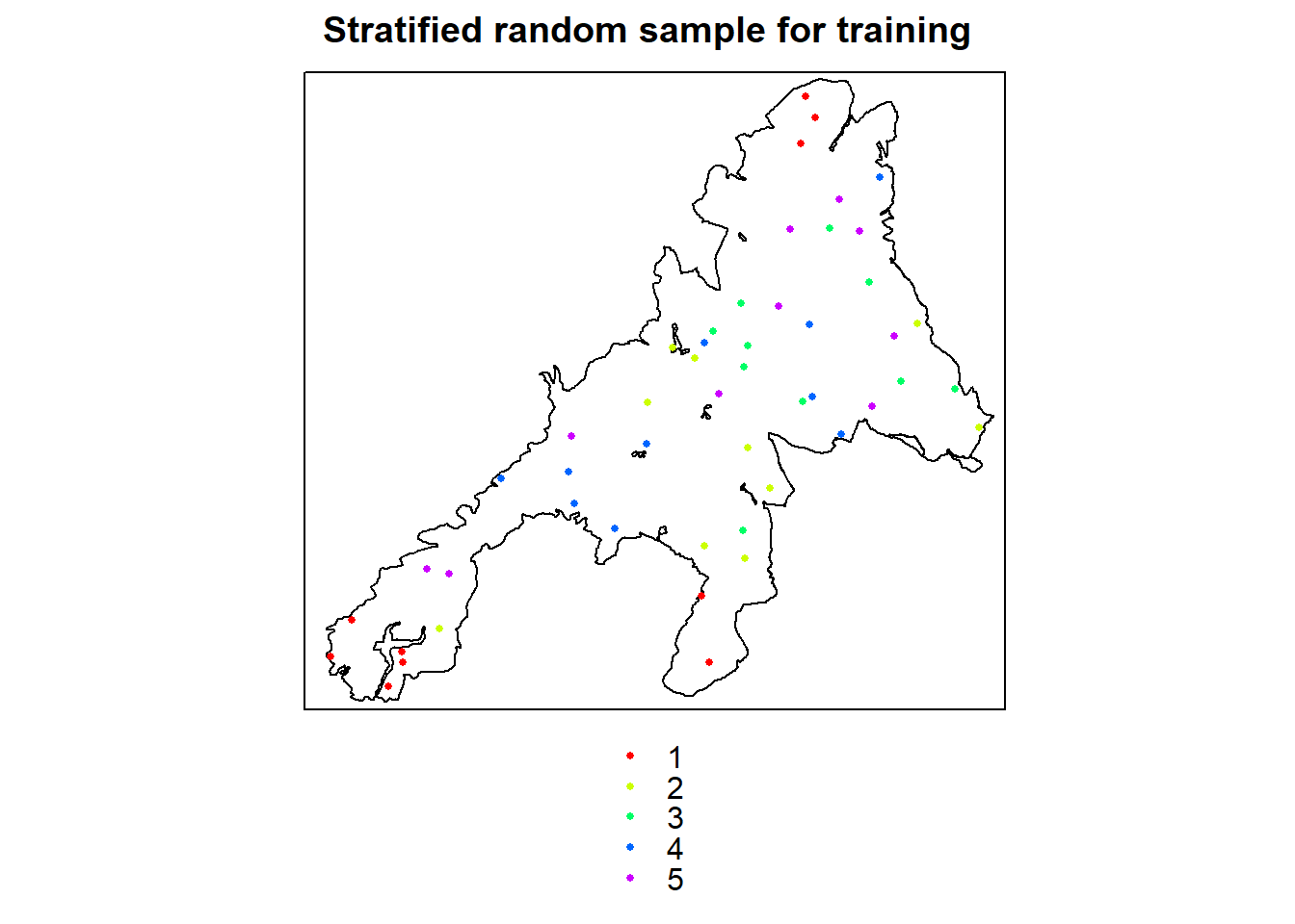
# Create a training data set by extracting the mean value of all pixels touching
# a buffered area with 13m around the plot center
train<-raster::extract(s2,samples,sp=T,buffer=13,fun='mean')
mapview(train, zcol="class",
        map.types = c("Esri.WorldShadedRelief", "OpenStreetMap.DE"))+
  mapview(np_boundary,alpha.regions = 0.2, aplha = 1)

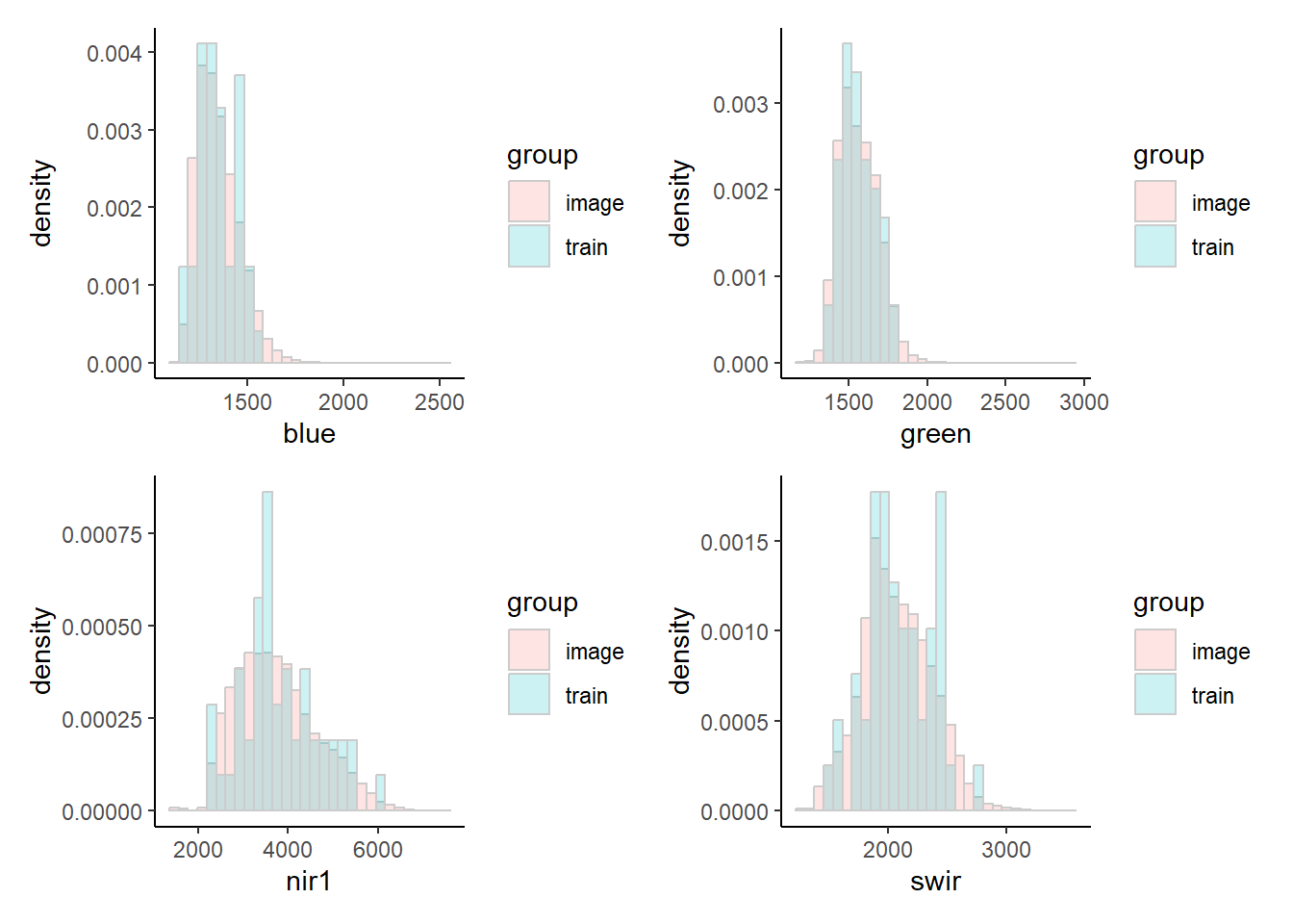
Compare the pixel value range between the sample and the image

image.sample<-raster::sampleRandom(s2,size=100000)
image.sample<- as.data.frame(image.sample)
image.sample$group<-'image'

train.df<- train@data[,names(s2)]
train.df$group<-'train'

df <- rbind(image.sample,train.df)

blue <-ggplot(df, aes(blue,fill=group)) + theme_classic()+
        geom_histogram(
        aes(y=after_stat(density)),alpha=0.2, color='gray80',
        position='identity',bins=30)

green <-ggplot(df, aes(green,fill=group)) + theme_classic()+
        geom_histogram(
        aes(y=after_stat(density)),alpha=0.2, color='gray80',
        position='identity',bins=30)

nir1<-ggplot(df, aes(nir1,fill=group)) + theme_classic()+
      geom_histogram(
      aes(y=after_stat(density)),alpha=0.2, color='gray80',
      position='identity',bins=30)

swir<-ggplot(df, aes(swir,fill=group)) + theme_classic()+
      geom_histogram(
      aes(y=after_stat(density)),alpha=0.2, color='gray80',
      position='identity',bins=30)

blue+green+nir1+swir+plot_layout(ncol=2)